Modeling Resilience: A Computational Exploration of Option B

Option B, by Sheryl Sandberg and Adam Grant, asks what people can build when the life they expected is no longer available. Reading it sent me toward a very engineer-shaped question: what would I have to assume to draw that process as a curve?

A dangerous question, if you forget that you drew the curve.

This is a Bayesian modeling exercise with 50 synthetic individuals. It explores the consequences of assumptions inspired by the book. It does not measure real recovery, validate the book's psychological claims, or predict anyone's future.

The interesting part is making the assumptions visible enough to argue with.

Build a small world

Each simulated individual has a stable “Option A” period, a disruptive event, and an “Option B” trajectory afterward. The generator assigns:

A baseline level, k_option_a_level.
An event-severity score, trauma_severity.
Resilience and support scores, combined into coping_resources_score, or CR.

The vertical axis is a synthetic functioning score. Calling it “skill” in a plot does not make it a validated measure of well-being. Those would be different constructs in a real study and would need separate definitions and measurements.

I designed the generator to produce different paths: lower plateaus, partial returns, returns to baseline, and some trajectories above baseline. In this toy world, coping resources affect those paths because the generating rules say they do. A trajectory above baseline is a numerical property of this score; it is not, by itself, evidence of post-traumatic growth.

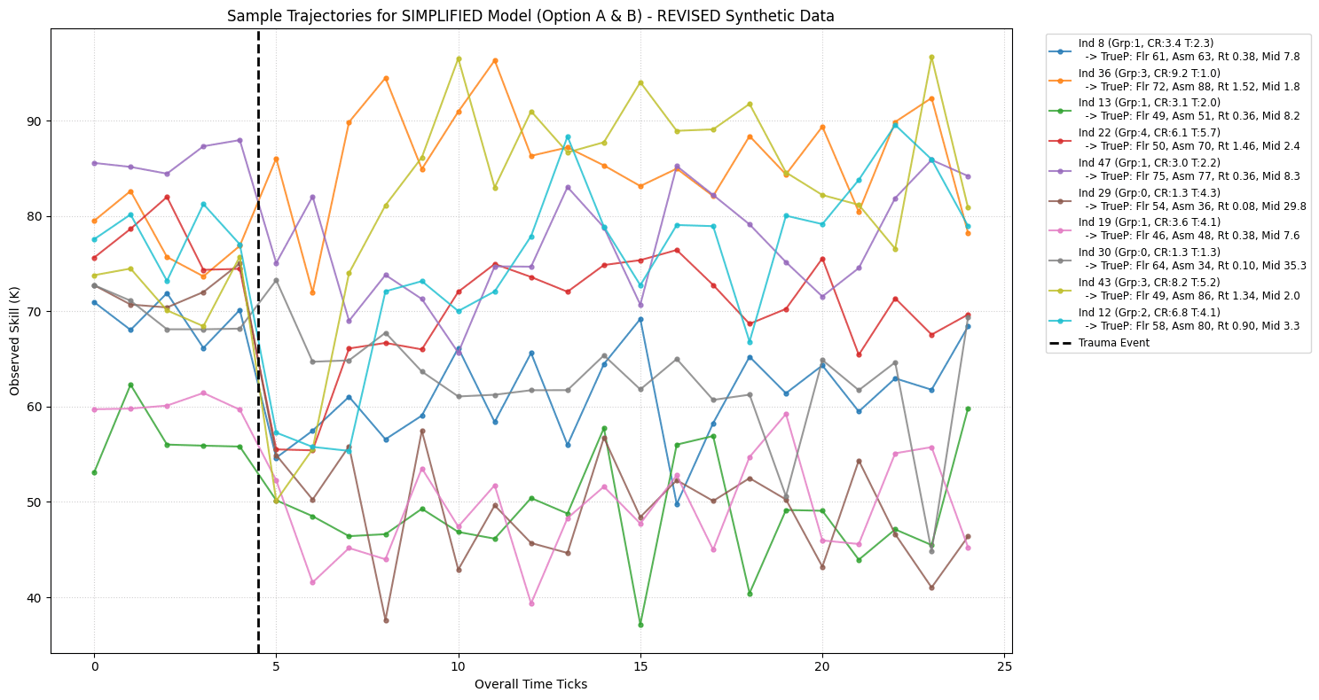Generated trajectories for a selection of synthetic individuals

Figure 1. Synthetic observations before and after the simulated event. Variation here comes from the generator, not a study of people.

Give the curve four moving parts

The model uses a logistic curve for individual $i$ at time $t$ :

\mu_{B_{it}} = K_{Floor_i} + \frac{K_{Asymptote_i} - K_{Floor_i}}{1 + \exp(-Rate_i (Time_{it} - Midpoint_i))}.

Read it through four parameters:

Parameter	What it controls in this model
$K_{Floor_i}$	Lower limiting level of the curve
$K_{Asymptote_i}$	Upper limiting level, when it exceeds the floor
$Rate_i$	How sharply the transition occurs
$Midpoint_i$	When the curve is halfway between its limiting levels

A detail matters: the floor is not generally the value at the event time. Substituting $t=0$ still leaves a positive logistic term. If we want a specific immediate drop, we must parameterize that initial value explicitly or check that the approximation is adequate.

With positive rate and an asymptote above the floor, the mean curve rises monotonically. That is a substantial assumption. It cannot represent repeated setbacks, several recovery phases, or lasting oscillations without changing the model. Noise around a smooth curve is not a substitute for modeling those mechanisms.

The observation model places a Normal distribution around $\mu_{B_{it}}$ :

K_{B_{it}}\sim\mathcal{N}(\mu_{B_{it}},\sigma_{K_B}^2).

Normal noise is convenient, but it can produce values outside a bounded score's range. If the score has real limits, the likelihood needs to respect them.

What makes it hierarchical?

Instead of fitting an unrelated curve to each individual, the PyMC model connects their parameters through shared relationships with baseline, severity, and CR. Individual variation can coexist with population-level parameters. This is partial pooling: a short, noisy trajectory can borrow information from the others, subject to the model's assumptions.

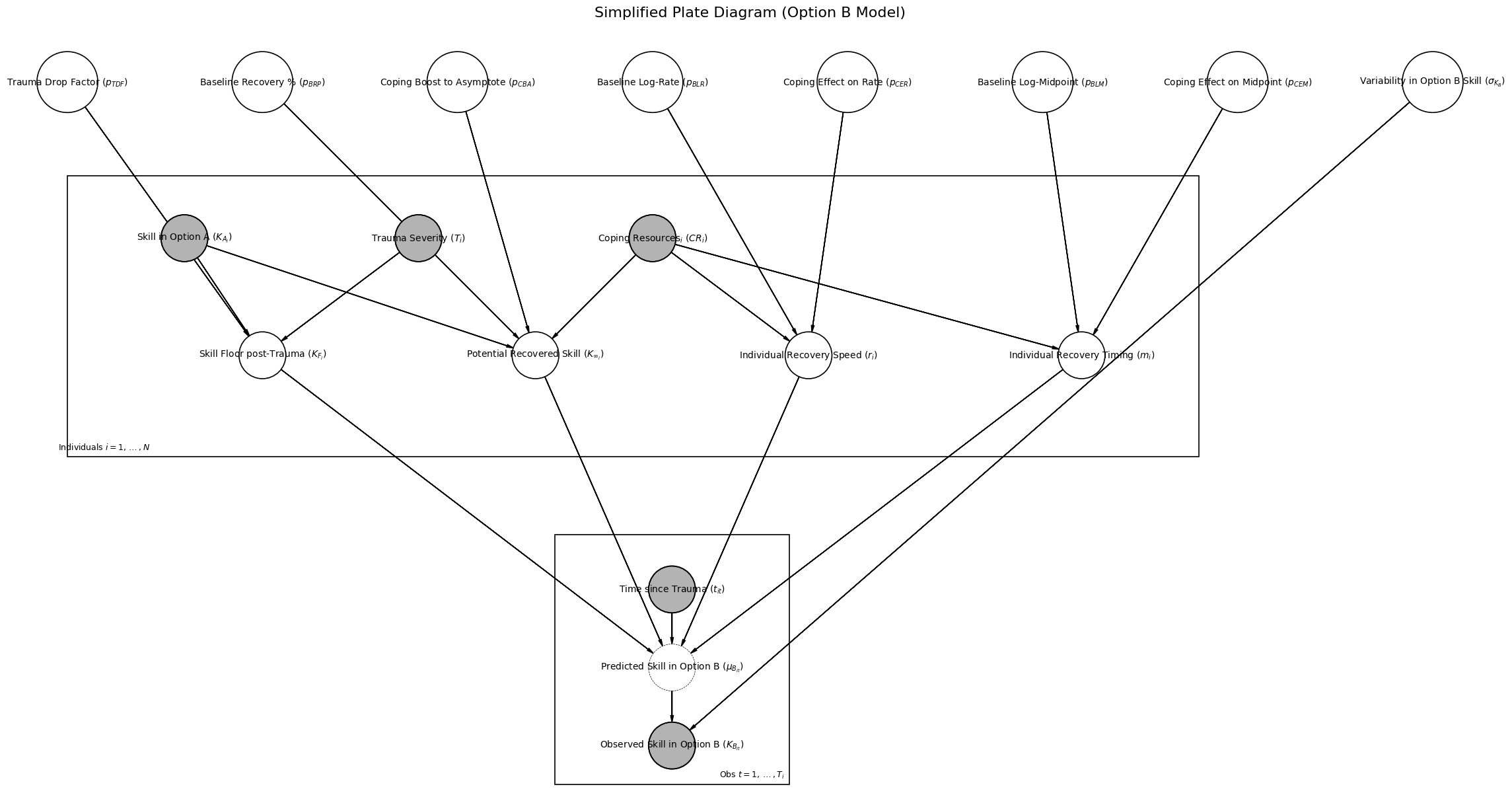Dependencies and repeated individual-level structure in the model

Figure 2. The plate diagram organizes the assumed dependencies. An arrow is a modeling choice; fitting synthetic observations does not establish that it is a causal relationship in people.

Read the parameters without overreading the result

The following numbers illustrate the scale of the model's terms. They are not clinical effect estimates, and without posterior intervals and diagnostics they should not be presented as established fitted effects.

For a baseline of 80, severity 5, and drop factor 0.06, a proposed floor calculation is:

80(1-5\times0.06)=56.

That tells us what this rule does. It also exposes a constraint: an unrestricted severity score could make the floor negative. The generator and parameter bounds need to prevent values the score cannot represent.

For the later limiting level, suppose a baseline-recovery fraction is 0.80 and a coping coefficient is 0.07. At normalized $CR=0.8$ :

K_{Asymptote}=80(0.80+0.07\times0.8)=68.48.

The coping term adds 4.48 points under these assumptions. It does not show that raising someone's support score by a unit would cause that improvement. Combining resilience and support into one score also prevents this model from identifying their separate contributions.

For rate and midpoint, log-scale coefficients need equally careful interpretation. If:

\log r_i=b_r+0.10CR_i,\qquad \log m_i=b_m-0.12CR_i,

then one unit of CR multiplies the rate by $e^{0.10}\approx1.105$ and the midpoint by $e^{-0.12}\approx0.887$ . The units matter: moving from 0 to 1 on a normalized score is its entire range, not one point on a ten-point questionnaire.

A noise standard deviation of 5 means observations vary around the modeled mean on that synthetic scale. It does not reveal a universal amount of variability in human recovery.

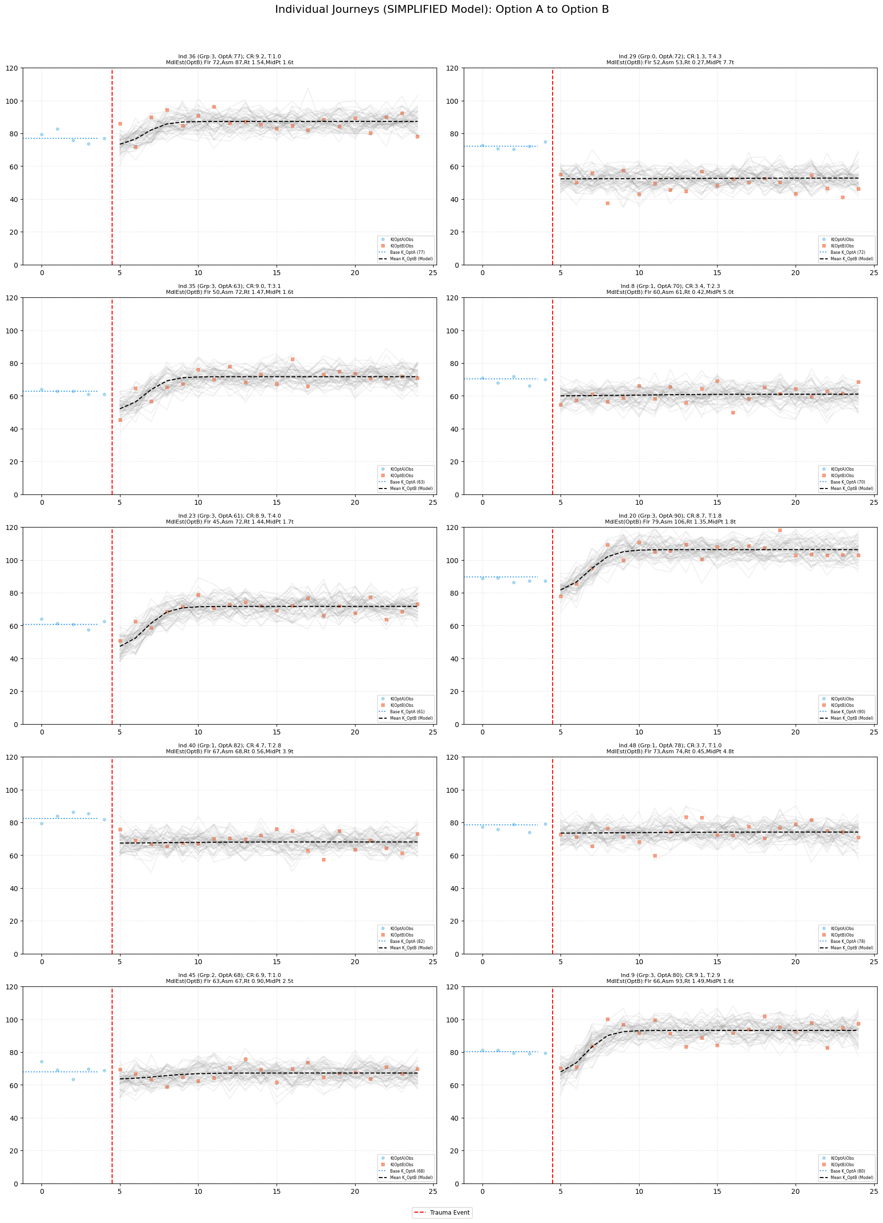Fitted curves and uncertainty for selected synthetic trajectories

Figure 3. Fits to synthetic trajectories. A close fit is evidence about this model and these generated observations. It is not independent confirmation of the psychological assumptions used to generate them.

The test that makes simulation useful

If I program support to improve the outcome, generate data, and recover a positive support coefficient, I have not discovered that support helps people. I have checked whether my inference machinery can recover a relationship I put into its world.

That is useful work when we ask the right questions:

Parameter recovery: can the model recover the known generating values across repeated simulated datasets, with appropriate uncertainty?
Identifiability: can short trajectories distinguish a slow rise toward a high plateau from a fast rise toward a low one?
Sensitivity: do the conclusions change sharply with priors, score normalization, or the assumed curve family?
Misspecification: what happens when the generator includes another setback or a non-logistic path?
Inference checks: do the chains mix, are effective sample sizes adequate, and are there divergent transitions or posterior predictive failures?

These are checks to perform, not results this post claims to have completed. A smooth black line on a chart does not answer them.

What would move this beyond the toy world?

More elaborate synthetic stories can test more elaborate assumptions. Generating those stories with an LLM does not turn them into independent evidence about people.

Moving beyond simulation requires longitudinal observations, clear definitions of the outcomes, and a study design that addresses missing data and confounding. Even a good predictive fit would not automatically identify the causal effect of support or resilience.

For this commute-sized experiment, the payoff is more modest and more concrete: the code forces me to say what “faster,” “higher,” and “more support” mean. Then it lets me see what those choices imply—and where they break.

The model does not tell us how a person ought to recover. It gives us a small world in which our assumptions have nowhere to hide.

Explore the computational notebook on Google Colab. The notebook is the original experiment; the distinctions and proposed checks above clarify how to interpret it.

The Power of the "Panic Button"
October 2, 2025
A practical leadership principle: give people a credible way to ask for help, revisit scope, or stop an experiment—and make that option work when they use it.