- Authors

- Name
- هاني الشاطر
Five restaurants are near your home. One of them is probably the best.
If their true quality was written on the door, the problem would be boring:
Read the numbers. Sort. Pick the largest.
But the numbers are not written anywhere. You have to discover them by eating. One dinner tells you something, but never the whole truth. Perhaps the chef had a bad night. Perhaps you ordered badly. Perhaps a usually average place served its best dish. Perhaps the excellent place had one terrible night.
Each restaurant has a real average quality . The value is hidden. A dinner is one noisy observation. You need enough evidence to order the restaurants without spending all your dinners on bad ones.
That creates the trade-off: exploit what currently looks best, or explore a restaurant whose quality is still unclear. Explore too little and an early lucky dinner can lock you into the wrong answer. Explore too much and you keep paying for mediocre meals after the answer is mostly clear.
The question becomes:
Where should the next try go?
That explore/exploit trade-off is the broader bandit problem. The action can be a restaurant, a road segment, a product candidate, a seller, an ad, a model, or a match. The structure of the decision may be known; the values that make one choice better than another are learned by spending attempts.
To find a shortest path through a city, the graph may be known while travel times on its edges are uncertain and variable. You do not merely run Dijkstra on fixed weights; driving a road is how you learn its weight.
To match customers with experts, the feasible matches may be known while the quality of each pairing is not. Every match teaches you something about preferences and compatibility, but it also uses an opportunity.
In all of these cases, the decision structure is known. The actions, constraints, and objective are clear. What is unknown are the parameters that determine which solution is best.
So before naming algorithms, separate two things:
- The decision structure — what you are allowed to choose.
- The feedback channel — what the world tells you after you choose.
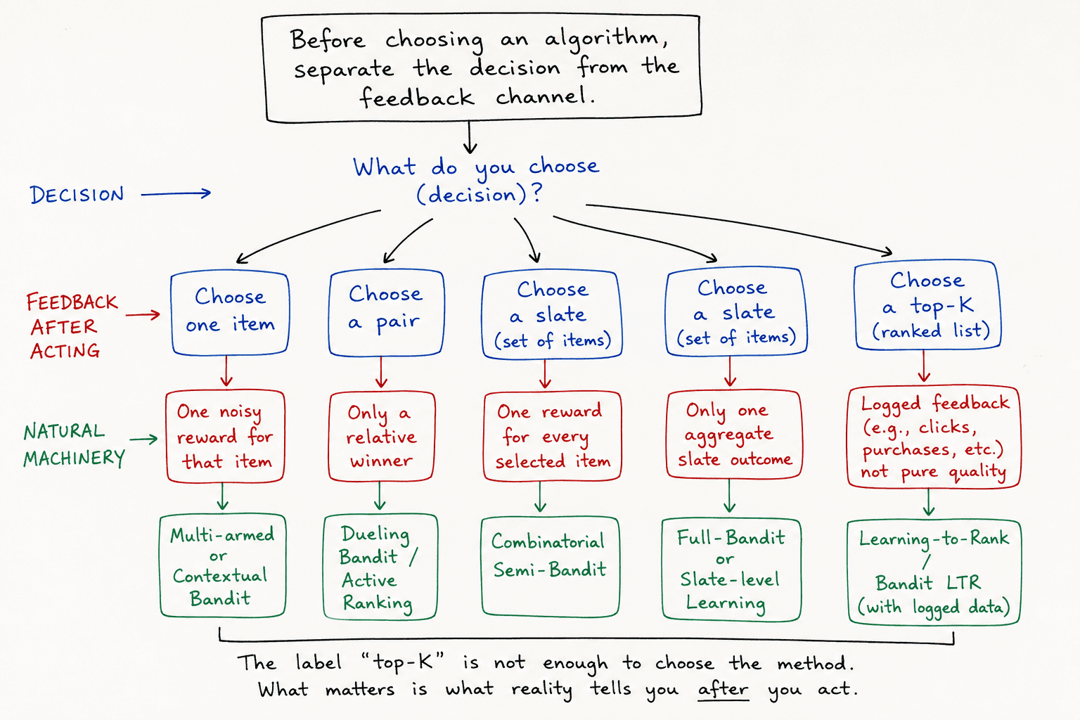
“Top-K” is not enough to choose the method. What matters is what reality tells you after the action.
Part I — The multi-armed bandit: choosing dinner
The restaurant problem has an old name: a multi-armed bandit. The casino metaphor is ugly, but the loop is useful.
Each restaurant is an arm. A visit is a pull. The dinner is the reward.
The catch is missing data. You choose one place, observe one noisy outcome, and the other four outcomes remain imaginary.
That missing information is the whole game.
Regret: the hidden tax of ignorance
If the sushi place is truly best and you eat somewhere weaker tonight, you paid a hidden tax. You may still have had a fine dinner, but compared with the best available dinner, you left quality on the table. Bandit theory calls that tax regret:
The formula is just bookkeeping. Each night, compare the place you chose, , with the best hidden average, . Add up the gap.
Regret comes from two opposite mistakes.
Commit too early, and one lucky ramen night can crown the wrong winner. Explore forever, and you keep buying mediocre dinners after the answer is mostly obvious.
A bandit policy is the rule that chooses the next pull. In practice, it is a rule for spending ignorance: which uncertainty is still worth paying for?
Before naming the algorithms, try the decision.
Use the demo to feel the trade-off before the algorithms show up.
Pick restaurants for a few dozen nights. Watch what happens when you trust early luck too much, and what happens when you keep sampling places that are clearly behind.
The lesson is the shape of the problem: exploration is useful only while it can still change the decision.
Four ways to spend uncertainty
ε-greedy. Most nights, go to the place that currently looks best. Every so often, ignore your notes and try a random place. That random night protects you from an early mistake, but it has a dumb habit: even after the winner is obvious, ε-greedy keeps paying the exploration tax.
UCB1 — optimism in the face of uncertainty. Score each arm by
and choose the largest score.
Here:
- is the total number of trials so far.
- is how many times arm has been tried.
- is the observed average reward of arm .
The second term,
is the exploration bonus.
It is large when is small and shrinks as evidence accumulates. UCB does not explore randomly. It explores where being wrong could still matter.
KL-UCB. UCB1 uses a generic confidence radius. KL-UCB uses a Bernoulli-shaped one.
For click/no-click or purchase/no-purchase feedback, it scores an arm by the largest plausible success rate in such that
Here KL is the statistical distance between the observed Bernoulli rate and the candidate rate .
The constraint says: choose the highest optimistic value that is still plausible under the observed Bernoulli data.
The move from 2% to 5% is not statistically the same as the move from 50% to 53%, even though both are three percentage points. KL-UCB respects that geometry.
Thompson sampling — let your beliefs race. Keep a whole distribution of possible qualities for each restaurant, not just one average. Each night, draw one plausible quality from every restaurant's belief and go to the highest draw.
A barely tried restaurant has a wide belief, so it sometimes draws high and earns another visit. A known-bad restaurant has a narrow low belief, so it almost never wins the draw. Nobody says “explore now.” Exploration falls out of uncertainty.
The hard case is when the top two restaurants are close.
Pure exploitation can crown the wrong winner after a lucky early meal. ε-greedy avoids some of that by forcing random exploration, then keeps paying the random tax after it has become less useful. UCB1 and KL-UCB spend more of their exploration on under-tested arms. Thompson sampling does the same through posterior samples rather than an explicit bonus.
KL-UCB is useful when the reward is close to Bernoulli, such as clicks or purchases. The catch is production feedback: if clicks are delayed, rank-biased, or mixed with presentation effects, the sharper bound can become fake precision.
Click to reveal: compact Bernoulli-bandit code
import math
import numpy as np


def bernoulli_kl(p, q):
    eps = 1e-12
    p = min(1 - eps, max(eps, p))
    q = min(1 - eps, max(eps, q))
    return p * math.log(p / q) + (1 - p) * math.log((1 - p) / (1 - q))


def kl_ucb(mean, pulls, t, c=3.0):
    if mean >= 1.0:
        return 1.0

    budget = (math.log(max(t, 2)) + c * math.log(math.log(max(t, 3)))) / pulls
    low, high = mean, 1.0 - 1e-12

    for _ in range(32):
        candidate = (low + high) / 2
        if bernoulli_kl(mean, candidate) <= budget:
            low = candidate
        else:
            high = candidate
    return low


def choose_arm(successes, pulls, t, policy, rng):
    unseen = np.flatnonzero(pulls == 0)
    if len(unseen):
        return int(rng.choice(unseen))

    means = successes / pulls

    if policy == "epsilon_greedy":
        return int(rng.integers(len(pulls))) if rng.random() < 0.10 else int(np.argmax(means))

    if policy == "ucb1":
        scores = means + np.sqrt(2.0 * np.log(t) / pulls)
        return int(np.argmax(scores))

    if policy == "kl_ucb":
        scores = np.array([kl_ucb(means[a], pulls[a], t) for a in range(len(pulls))])
        return int(np.argmax(scores))

    if policy == "thompson":
        samples = rng.beta(1 + successes, 1 + pulls - successes)
        return int(np.argmax(samples))


def update(successes, pulls, arm, reward):
    pulls[arm] += 1
    successes[arm] += reward
The next useful pull is usually the one that can still change your mind.
Context changes the answer
The plain bandit gives each restaurant one number: . That is clean, and often false.
A quick lunch, a family dinner, a work meal, guests visiting from out of town, and a rainy solo evening are not the same decision. A restaurant can be wrong for one and perfect for another. The point of context is to stop averaging those cases together.
That is the point of a contextual bandit: see the situation first, then choose.
In a linear contextual bandit, the situation is a feature vector . For dinner, features might be things like quick, quiet, cheap, child-friendly, spicy, or suitable for a group. Each arm has a response vector that says how much those features matter for that arm.
The predicted reward is
The dot product asks: how well does this arm fit this situation?
This is where context helps. A dinner on one quick-budget night is not only evidence about that exact night. It also updates the coefficients attached to quick and budget, so it informs other contexts that share those features. The model learns from correlated contexts instead of treating every situation as unrelated.
LinUCB is UCB with this linear model inside it. For each arm, it keeps the statistics needed to estimate :
Here records which contexts arm has been tried in, and records the rewards seen in those contexts. Together they give
Then it chooses the arm with the largest optimistic score:
The first term is predicted reward in the current context. The second term is uncertainty in this part of the context space. If the model has little evidence there, the bonus is larger. If it has seen many similar contexts, the bonus shrinks.
The unknown has moved from average quality to situational fit:
What situations is this restaurant good for?
Context must be known before the choice. If you only learn it after the meal, click, purchase, delivery, or complaint, it is feedback — not context.
In the demo, the non-contextual policy keeps one average per restaurant. LinUCB conditions on the situation first.
When the same restaurant is good in one context and bad in another, the contextual policy should lose less regret because it stops pooling incompatible dinners.
Click to reveal: disjoint LinUCB in NumPy
import numpy as np


class DisjointLinUCB:
    def __init__(self, n_arms, dim, alpha=0.8, l2=1.0):
        self.alpha = alpha
        self.A = [l2 * np.eye(dim) for _ in range(n_arms)]
        self.b = [np.zeros(dim) for _ in range(n_arms)]

    def choose_arm(self, x):
        scores = []
        for A_a, b_a in zip(self.A, self.b):
            theta_a = np.linalg.solve(A_a, b_a)
            predicted_reward = x @ theta_a
            uncertainty = np.sqrt(x @ np.linalg.solve(A_a, x))
            scores.append(predicted_reward + self.alpha * uncertainty)
        return int(np.argmax(scores))

    def update(self, arm, x, reward):
        self.A[arm] += np.outer(x, x)
        self.b[arm] += reward * x


# x must contain only information known before the action.
# Example: [1, is_lunch, is_family_dinner, is_raining, mobile_user].
arm = policy.choose_arm(x_t)
reward = observe_reward(arm)
policy.update(arm, x_t, reward)
Sometimes the clean number never arrives.
Sports gives you matches. LLM evaluation gives you preferences. A judge may struggle to assign an absolute score, but it can still compare two outputs.
The feedback becomes pairwise: choose two items, observe a winner.
Part II — Pairwise ranking: when the arm is a match
The action has changed.
Part I chose one arm and received one reward. Here the unit of evidence is a match: choose two candidates, observe which one wins.
A match is a noisy comparison. Strong players usually beat weak ones. Close players need rematches because one result settles little.
With candidates, there are possible pairs. Comparing everything is already expensive at a small scale, and impossible at product scale.
The table improves only when the next comparison has value.
If a new candidate beats the current champion, testing it only against weak candidates next is mostly ceremony. Useful matches sit near unresolved boundaries.
So the question becomes: which match should happen next?
This is sorting with an unreliable comparator.
In a textbook sort, one comparison resolves the order of two items. Here, one match is only evidence.
The action is a pair. The feedback is one bit: who won?
No absolute quality number.
A common way to make this usable is Bradley-Terry.
Assume each item has one hidden skill score, and win probabilities come from score differences:
Equal scores give a 50/50 match. A large gap gives a near-certain result. The absolute scale is arbitrary; only differences matter.
The payoff is transfer. If A repeatedly beats B, and B repeatedly beats C, the model already has evidence about A versus C.
The boundary is expensive. Up to constants, distinguishing a small skill gap with confidence takes roughly
comparisons.
Big gaps settle quickly. Near ties eat the budget.
From pairwise feedback to skill ratings
Batch fit. Given all matches so far, fit the Bradley-Terry scores that make the observed winners most likely.
If A beat B many times, the fit pushes A above B until roughly matches the history. If B beat C many times, B rises above C. Because the model has one shared scale, those facts also move A relative to C even if A and C never played.
One standard batch update works with positive strengths instead of log-scores directly. Let
Then a Bradley-Terry MM update is
After each pass, normalize the strengths and return . Bradley-Terry only cares about relative strength; multiplying every by the same constant changes nothing.
Sort the fitted scores and you have a ranking. Clean. Expensive. Refitting from scratch after every match does not scale.
Online fit: Elo. Elo is the streaming version. Keep one rating per player and update it after each match.
A win moves rating from loser to winner. The move is bigger when the result was surprising.
Beat the world champion and you should gain a lot. Beat a beginner and you should gain almost nothing. Lose to a much weaker player and your rating should fall sharply.
One way to write that update is as a logistic-regression step. If beats :
Here is the model’s pre-match probability that beats . The update is surprise: .
If was already a heavy favourite, the move is small. If was an underdog, the move is large.
Click to reveal: Bradley–Terry batch fitting and online Elo
import numpy as np


def fit_bradley_terry_mm(wins, iterations=100, eps=1e-9):
    """
    wins[i, j] is the number of times item i beat item j.

    MM update in positive strengths:
        strength_i <- wins_i / sum_j n_ij / (strength_i + strength_j)

    Returns log-strengths; sorting them gives the Bradley–Terry ranking.
    """
    wins = np.asarray(wins, dtype=float)
    pair_games = wins + wins.T
    total_wins = wins.sum(axis=1)
    n_items = len(wins)
    strength = np.ones(n_items)

    for _ in range(iterations):
        updated = strength.copy()
        for i in range(n_items):
            denominator = 0.0
            for j in range(n_items):
                if i != j and pair_games[i, j] > 0:
                    denominator += pair_games[i, j] / (strength[i] + strength[j])

            if denominator > 0:
                updated[i] = max(total_wins[i], eps) / denominator

        # Bradley–Terry is identifiable only up to an additive constant in log-space.
        updated /= np.exp(np.mean(np.log(np.maximum(updated, eps))))
        strength = updated

    return np.log(np.maximum(strength, eps))


def elo_update(rating, i, j, winner, learning_rate=0.25):
    """One online logistic-regression step after i versus j."""
    p_i_wins = 1.0 / (1.0 + np.exp(-(rating[i] - rating[j])))
    target_i = 1.0 if winner == i else 0.0
    delta = learning_rate * (target_i - p_i_wins)

    rating[i] += delta
    rating[j] -= delta
    return rating


# Batch: scores = fit_bradley_terry_mm(wins)
# Online: rating = elo_update(rating, i, j, winner)
The loop is:
estimate skills from matches → read off the ranking by sorting → schedule the next match.
Where to spend the matches
The next match should be one where the result can still move the table.
A lopsided match usually confirms the obvious. If #1 beats #8, the table barely moves.
A close match does real work. Either result is plausible. Either result teaches something about the local order.
A useful scheduler looks for pairs that are both close and under-sampled.
Random chooses any pair.
Round-robin chooses the least-played pair, .
Ladder compares neighbours in the current table.
Active spends the next match where rank uncertainty is highest:
The curve is mean top-5 recall across repeated leagues: how many of the true best five candidates have entered the estimated best five. The early part matters most, because with enough matches most reasonable schedulers eventually catch up.
Set the table to you scout (click 2). Pick a match, inspect how the ranking moves, then pick again.
The easy-looking matches are usually the least useful. The valuable matches are the ones where either result would teach you something.
Why the candidate pool must be wider than K
Often you do not need the whole ranking. You only need the best K.
If , the cutline is the current boundary around rank 100: the place where inclusion in the set is still up for grabs.
Comparing only the current top-K freezes early mistakes.
- A genuinely top-K item currently sitting at K+1 receives no matches and has no path back into contention.
- Inside a settled top-K, comparisons are often lopsided; the cutline does not move.
- If the top group is isolated from the field, “K-th best” loses its anchor.
The fix is a candidate band around the cutline.
Keep sampling items whose uncertainty still overlaps the K-th position. Narrow the band only when evidence pushes them out.
Click to reveal: active matching around a top-K cutline
import numpy as np


def candidate_band(scores, score_se, k, z=1.96):
    """
    Keep candidates whose confidence intervals overlap the current K-th item.
    score_se can come from a Hessian approximation, a bootstrap, or a posterior.
    """
    order = np.argsort(-scores)
    cutline_item = order[k - 1]
    cutline_low = scores[cutline_item] - z * score_se[cutline_item]
    cutline_high = scores[cutline_item] + z * score_se[cutline_item]

    lower = scores - z * score_se
    upper = scores + z * score_se
    band = np.flatnonzero((upper >= cutline_low) & (lower <= cutline_high))

    # Keep enough local rivals even when the intervals are overconfident early on.
    local = order[max(0, k - 4):min(len(scores), k + 4)]
    return np.unique(np.concatenate([band, local]))


def choose_active_pair(scores, score_se, pair_games, candidates):
    """Prefer uncertain, close pairs inside the cutline candidate band."""
    best_pair = None
    best_value = -np.inf

    for left in range(len(candidates)):
        for right in range(left + 1, len(candidates)):
            i, j = candidates[left], candidates[right]

            # Lightweight heuristic. A full BTL fit should use uncertainty
            # of the difference s_i - s_j, including covariance.
            pair_se = np.sqrt(score_se[i] ** 2 + score_se[j] ** 2)
            standardized_gap = abs(scores[i] - scores[j]) / (pair_se + 1e-9)
            boundary_value = 1.0 / (1.0 + standardized_gap)
            pair_uncertainty = 1.0 / np.sqrt(pair_games[i, j] + 1.0)
            value = boundary_value * pair_uncertainty

            if value > best_value:
                best_value = value
                best_pair = (i, j)

    return best_pair


# At every round:
# band = candidate_band(elo_rating, score_se, k=100)
# i, j = choose_active_pair(elo_rating, score_se, pair_games, band)
# winner = observe_comparison(i, j)
# elo_rating = elo_update(elo_rating, i, j, winner)
The implementation above is only the principle. Keep a band around the cutline; use whatever uncertainty estimate your model can support to decide who still belongs.
With 10,000 players there are about 50 million possible pairs. Exhaustive comparison is not a plan.
Use an online estimator such as Elo and an adaptive scheduler that focuses comparisons near the K-th rating. The metric is recall@100: how much of the true top-100 appears in the estimated top-100.
In this synthetic setting, random pairing wastes matches far from the cutline. Adaptive matching recovers most of the top 100 in tens of thousands of matches instead of enumerating fifty million pairs.
It wins by spending matches where membership is still uncertain. The exact count depends on the gaps around rank 100, outcome noise, model fit, and the stopping rule.
Part III — Combinatorial semi-bandits: when the action is a slate
So far, one round bought one observation: one dinner, one match.
Now one round buys a slate.
Part III chooses several items at once.
A product surface rarely asks for one item. It asks for a list: top 10 products, 12 snippets, 20 candidates, a page of recommendations.
Pairwise ranking buys a global order, but the bill is O(n²). A hundred items is already about five thousand pairs. A million is dead.
Part II reduced the bill by spending comparisons near the cutline. Part III uses a different lever: select a slate, observe feedback on the selected items, and update only those items.
That is a combinatorial semi-bandit: the action is a set, and feedback decomposes over the pieces you actually chose.
Part III.1 — When the score has to be manufactured
The policy is optimism again, one level up.
Give each item an estimate and an uncertainty bonus, then select the top-K by optimistic score:
Here is the current reward estimate and is how many times item has received usable feedback.
A high estimate earns a slate seat. High uncertainty can earn one too. Each round: take the top-K by , observe one outcome per selected item, and update those items.
On a real surface, the additive-reward assumption is fragile — position bias, cannibalization, exposure, and presentation all leak in. But the base loop is still useful.
The hard question is where comes from.
- Direct reward. The world gives a number per item — click, watch time, benchmark score. Then the policy below is enough.
- Only comparisons. The world gives “A beat B.” Comb-UCB needs a per-item reward, so raw pairwise wins need a scoring layer first.
In the second case, you manufacture a reward proxy.
Run small tournaments: ask one judge to rank 10–20 items, break the ranking into pairwise wins, and fit Bradley-Terry as in Part II. The tournament turns local comparisons into a latent on a shared scale.
That score is not ground truth. It is the current best utility estimate used to allocate the next round of judgment.
Part II creates the score. Part III decides where to spend the next slate.
Click to reveal: combinatorial UCB with per-item rewards
import numpy as np


class CombinatorialUCB:
    def __init__(self, n_items, exploration=1.0):
        self.reward_sum = np.zeros(n_items)
        self.pulls = np.zeros(n_items, dtype=np.int64)
        self.exploration = exploration

    def select_slate(self, k, t):
        means = np.divide(
            self.reward_sum,
            self.pulls,
            out=np.zeros_like(self.reward_sum),
            where=self.pulls > 0,
        )
        bonus = np.full_like(means, np.inf)
        seen = self.pulls > 0
        bonus[seen] = self.exploration * np.sqrt(np.log(max(t, 2)) / self.pulls[seen])
        scores = means + bonus

        # argpartition avoids sorting every item when k << n_items.
        slate = np.argpartition(scores, -k)[-k:]
        return slate[np.argsort(-scores[slate])]

    def update(self, slate, rewards):
        self.pulls[slate] += 1
        self.reward_sum[slate] += np.asarray(rewards)


slate = policy.select_slate(k=12, t=round_number)
rewards = observe_per_item_rewards(slate)  # one reward for every selected item
policy.update(slate, rewards)
Read the demo as a feedback-channel comparison.
Comb-UCB receives several direct rewards per round, one for each selected item. Bradley-Terry receives one comparison bit per duel, then fits a reusable global ranking.
Part III.2 — Mining reviews for the best line
Now use the same loop on a real pile: thousands of customer reviews, with the goal of surfacing a few noteworthy lines.
There is no natural per-item reward for a snippet: no click, no benchmark score, no clean scalar target. The available signal is judgment.
The semi-bandit decides which snippets deserve judgment next. Bradley-Terry turns those judgments into a score.
candidates = extract_snippets(reviews)        # large pool, no scores yet
score = {c: 0.0 for c in candidates}          # Bradley-Terry latent reward
pulls = {c: 0   for c in candidates}
pairs = []

for t in range(1, rounds + 1):
    # 1. SELECT an optimistic, diverse slate using current BT scores
    ucb   = {c: score[c] + C * sqrt(log(t + 1) / (pulls[c] + 1)) for c in candidates}
    slate = top_k_constrained(ucb, k=K, max_per_type=...)   # <= K, capped per type

    # 2. JUDGE: one listwise ranking of the slate -- a small tournament
    ranking = llm_rank(slate)               # "order these from best to worst"

    # 3. CALIBRATE: ranking -> pairwise wins -> refit Bradley-Terry
    pairs += ranking_to_pairs(ranking)      # i beats j for every i ranked above j
    score  = fit_bradley_terry(pairs)

    # 4. only judged items count as pulled
    for c in slate:
        pulls[c] += 1

best = sorted(candidates, key=lambda c: score[c], reverse=True)[:K]
Two things keep this away from the bill.
UCB selectivity spends judgment where the order is still in doubt and leaves the settled tail alone.
Listwise judging multiplies one call into many constraints: one ranking of K items yields pairwise wins. They are not independent observations, but they are still useful ordering constraints.
I ran this on a random sample of 1,500 reviews from the McAuley Amazon Reviews dataset. Before snippet extraction, I filtered to four- and five-star reviews. That left 114 candidate lines, , and eleven rounds.
The bill it did not pay:
| exhaustive pairwise | this run | |
|---|---|---|
| candidates | 114 | 114 |
| one full pass | 6,441 pairs | not taken |
| expensive judge calls | thousands | 22 |
| pairwise constraints | — | 2,582 |
| the dull tail | compared anyway | judged 0–1× |
The funniest lines it surfaced, by Bradley-Terry score (every line a verbatim review):
| Bradley-Terry | judged | the line |
|---|---|---|
| +4.05 | 11× | "3.6 Roentgen. Not great, not terrible." |
| +3.16 | 9× | "There is a reason more people have Amazon Prime than own guns in the United States." |
| +3.09 | 8× | "Thanks Amazon — if it was up to you, I would never have to leave my house. Unfortunately there are some inconveniences in my life, such as work." |
| +2.28 | 9× | "Only problem is they don't come through my door and start performing." |
| +5.22 | 1× | "…the best thing that ever happened to me. Family comes second." |
That last row is the failure mode optimism is meant to catch.
It has the highest fitted score after one judgment, which makes it interesting, not trustworthy. UCB should send it back for another test instead of crowning it.
The trustworthy line is the one judged eleven times. Highest score and highest score you believe are different questions. Ranking by alone answers the wrong one.
One production caveat: the optimizer optimizes the target you give it.
An earlier pass without the four-and-five-star filter surfaced only outrage — a wall of one-star delivery horror stories. The method did not discover “funny.” It followed the filter and the judge instruction.
Noteworthy and funny are choices you encode, not properties the optimizer finds on its own.
A short history of bandits
The basic problem is old: learn which uncertain option is best while losing as little as possible on the way. The language changed, the feedback channels multiplied, and the action space grew from one lever to whole slates and structured decisions. The core tension survived.
Probability matching: sample a plausible world, then act as though it were true.
Sequential allocation becomes the modern multi-armed-bandit question.
Regret lower bounds clarify the cost of learning; confidence bounds give a practical optimistic rule.
Contextual, dueling, ranking, and combinatorial versions make the feedback channel part of the problem definition.
The post follows that expansion: one reward becomes context-conditioned reward; then a pairwise win; then item-level feedback for a whole slate. The action changes, but so does what reality lets the learner observe.
Primary reading
- Thompson (1933), On the Likelihood that One Unknown Probability Exceeds Another.
- Robbins (1952), Some Aspects of the Sequential Design of Experiments.
- Lai and Robbins (1985), Asymptotically Efficient Adaptive Allocation Rules.
- Auer, Cesa-Bianchi, and Fischer (2002), Finite-Time Analysis of the Multiarmed Bandit Problem.
- Li, Chu, Langford, and Schapire (2010), A Contextual-Bandit Approach to Personalized News Article Recommendation.
- Yue and Joachims (2009), Interactively Optimizing Information Retrieval Systems as a Dueling Bandits Problem.
- Kveton et al. (2015), Tight Regret Bounds for Stochastic Combinatorial Semi-Bandits.
About the interactive demos: UCB1, KL-UCB, Thompson sampling, LinUCB, Bradley–Terry, Elo, and combinatorial semi-bandits correspond to established families above. The active-pairing scheduler, the cutline matcher, and the overlapping bootstrap-Elo leagues are explanatory heuristics built for this post; they are not claimed as canonical algorithms or theorem-optimal policies.